Neural Architecture Search

Introduction: What is NAS?

Neural Architecture Search (NAS) is an approach for automating the design of deep neural networks. Instead of relying on human intuition and trial-and-error, NAS algorithms explore a predefined search space to find architectures that perform well on a given task.

A typical NAS pipeline involves:

1. Search Space: Defines the types of operations and connections allowed.
2. Search Strategy: Determines how the space is explored (e.g., reinforcement learning, evolution, gradient descent).
3. Evaluation Strategy: Estimates the performance of candidate architectures.

---

DARTS: Differentiable Architecture Search

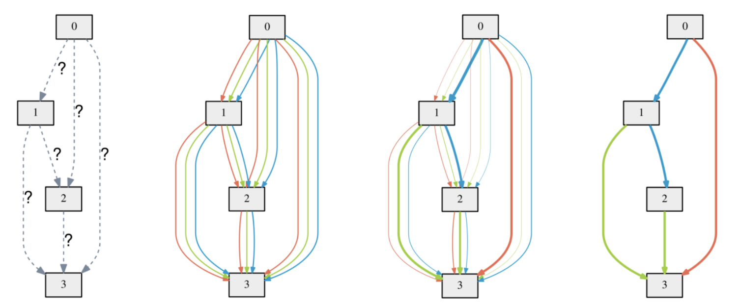
DARTS (2018) introduced a gradient-based NAS framework by relaxing the discrete architecture search space into a continuous one. Each operation between nodes is represented by a weighted mixture:

$$\bar{o}^{(i, j)}(x) = \sum_{o \in \mathcal{O}} \frac{\exp(\alpha_o^{(i,j)})}{\sum_{o' \in \mathcal{O}} \exp(\alpha_{o'}^{(i,j)})} \cdot o(x)$$

Here, $\alpha^{(i,j)}$ are architecture parameters learned via gradient descent.

This allows joint optimization of:

• $w$: network weights
• $\alpha$: architecture weights

via bi-level optimization:

$$\begin{aligned} w^*(\alpha) &= \arg\min_w \mathcal{L}_{\text{train}}(w, \alpha) \\ \alpha^* &= \arg\min_\alpha \mathcal{L}_{\text{val}}(w^*(\alpha), \alpha) \end{aligned}$$

How DARTS Optimization Works in Practice

Solving the bi-level optimization problem above directly is intractable. The inner optimization requires finding the optimal weights $w^*$ for every potential architecture $\alpha$, which would mean fully re-training the network every time we update $\alpha$. This is computationally prohibitive.

To overcome this, DARTS employs a two-part approximation:

1. Approximate $w^*$ with a Single Gradient Step

Instead of fully training the network to get $w^*$, DARTS approximates it using $w'$, which is the result of just a single training step:

$w' \approx w^*(\alpha) = w - \xi \nabla_w \mathcal{L}_{\text{train}}(w, \alpha)$

Here, $\xi$ is a learning rate for this single “inner” update. Now, the goal is to update $\alpha$ by calculating the gradient $\nabla_\alpha \mathcal{L}_{\text{val}}(w', \alpha)$.

2. Approximate the Hessian-vector Product with Finite Differences

Applying the chain rule to get the gradient for $\alpha$ introduces a second-order derivative (a Hessian matrix) that is also expensive to compute:

$\nabla_\alpha \mathcal{L}_{\text{val}}(w', \alpha) \approx \nabla_\alpha \mathcal{L}_{\text{val}}(w', \alpha) - \xi \nabla_{\alpha, w}^2 \mathcal{L}_{\text{train}}(w, \alpha) \nabla_{w'} \mathcal{L}_{\text{val}}(w', \alpha)$

The costly term is the Hessian-vector product $\nabla_{\alpha, w}^2 \mathcal{L}_{\text{train}} \cdot \nabla_{w'} \mathcal{L}_{\text{val}}$. DARTS sidesteps this by using a finite difference approximation:

$\nabla_{\alpha, w}^2 \mathcal{L}_{\text{train}}(w, \alpha) \nabla_{w'} \mathcal{L}_{\text{val}}(w', \alpha) \approx \frac{\nabla_\alpha \mathcal{L}_{\text{train}}(w^+, \alpha) - \nabla_\alpha \mathcal{L}_{\text{train}}(w^-, \alpha)}{2\epsilon}$

where $w^{\pm} = w \pm \epsilon \nabla_{w'} \mathcal{L}_{\text{val}}(w', \alpha)$, and $\epsilon$ is a small scalar. This allows estimating the architectural gradient with only two forward passes and two backward passes, avoiding the explicit Hessian computation.

By combining these approximations, DARTS can efficiently find a promising architecture. However, these approximations, while efficient, are also a source of instability and contribute to some of the issues listed below.

While efficient, DARTS suffers from issues like:

• Overfitting to weight-sharing artifacts
• Architecture collapse to trivial choices
• Lack of generalization guarantees

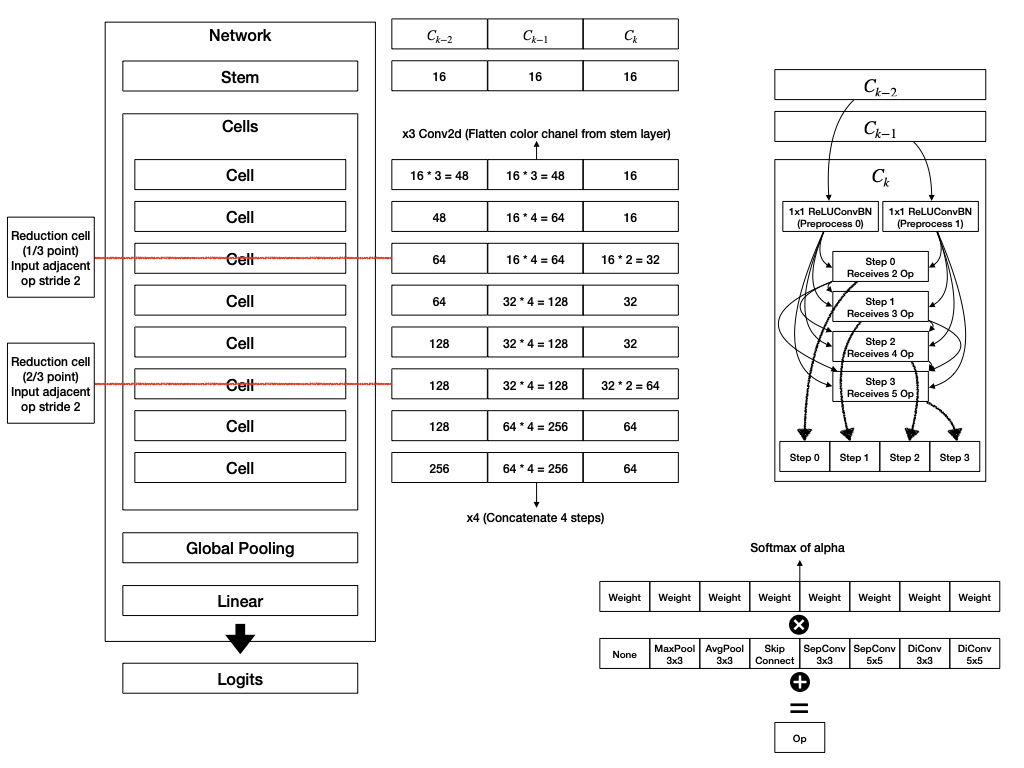
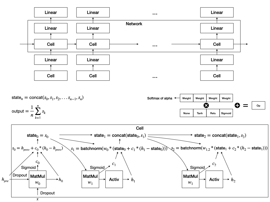
The figure below is a schematic of the architecture of DARTS for cnn and rnn restored based on the paper.

---

XNAS: NAS with Expert Advice (Nayman et al., 2019)

To overcome DARTS’ limitations, XNAS (Expert Advice NAS) frames NAS as an online learning problem using the Follow-the-Regularized-Leader (FTRL) algorithm. This provides theoretical guarantees and improved stability.

---

Key Idea

Treat each architecture as an expert, and use online learning with expert advice to learn a probability distribution over the experts (architectures).

• Let $\mathcal{A}$ be the set of all possible architectures (e.g., combinations of operations on a DAG).
• At each round $t$, the algorithm selects a distribution $p^{(t)}$ over $\mathcal{A}$.
• One architecture $a^{(t)} \sim p^{(t)}$ is sampled and trained.
• The resulting loss $l^{(t)}(a^{(t)})$ is used to update the distribution.

---

FTRL Objective

At each round $t$, FTRL chooses $p^{(t)}$ as:

$$p^{(t)} = \arg\min_{p \in \Delta} \left[ \sum_{s=1}^{t-1} \langle p, \ell^{(s)} \rangle + \frac{1}{\eta} R(p) \right]$$

• $\ell^{(s)}$: loss vector over all experts at round $s$
• $R(p)$: regularization term (e.g., negative entropy)
• $\eta$: learning rate
• $\Delta$: probability simplex over $\mathcal{A}$

This balances exploitation (low cumulative loss) and exploration (via regularization).

---

The Power of Exponentiated Gradient (EG) Update

A key difference from DARTS lies in how the architecture parameters are updated. The EG update rule in the algorithm, $v_{t,i} \leftarrow v_{t-1,i} \cdot \exp(\eta R_{t,i})$, seems different from standard gradient descent, but it’s actually its natural counterpart in the probability space.

Let’s see why.

In DARTS, updates are additive on the logits : $\alpha_{new} \leftarrow \alpha_{old} - \eta \nabla \mathcal{L}$

The unnormalized scores $v$ (before softmax) are typically $v = \exp(\alpha)$.
If we apply the gradient update to $\alpha$, the new scores become: $v_{new} = \exp(\alpha_{new}) = \exp(\alpha_{old} - \eta \nabla \mathcal{L})$

Using the property of exponents, this can be rewritten as: $v_{new} = \exp(\alpha_{old}) \cdot \exp(-\eta \nabla \mathcal{L}) = v_{old} \cdot \exp(-\eta \nabla \mathcal{L})$

Since the reward $R$ is defined as the negative loss gradient ($R = -\nabla \mathcal{L}$), we arrive at the EG update rule: $v_{new} \leftarrow v_{old} \cdot \exp(\eta R)$

This shows that an additive update on logits is equivalent to a multiplicative update on the unnormalized scores. By using this form directly, XNAS ensures that the update magnitude depends on the reward, not the current weight. This prevents experts with small weights from getting stuck and allows for more robust exploration.

---

Practical Implementation in XNAS

Directly enumerating all architectures is infeasible, so XNAS:

• Decomposes the architecture into local decisions (e.g., operation choices on each edge)

• Uses a product distribution over edges:

  Let $E$ be the set of edges, and each edge $e$ has candidate operations $\mathcal{O}_e$.

  Then:

  $$p(a) = \prod_{e \in E} p_e(o_e)$$

  where $p_e$ is the categorical distribution over $\mathcal{O}_e$.

• Updates each $p_e$ using the FTRL rule independently.

---

Online-to-Batch Conversion

After $T$ rounds of online training, the final architecture can be:

• Sampled from the learned distribution $p^{(T)}$
• Or chosen as the argmin of cumulative loss across rounds

---

Regret Guarantee

XNAS provides a regret bound of:

$$\text{Regret}_T \leq O\left( \sqrt{T \log |\mathcal{A}|} \right)$$

This means that the algorithm asymptotically performs as well as the best fixed architecture in hindsight.

---

Wipeout: Principled Pruning in XNAS

In the XNAS framework, Wipeout refers to a pruning mechanism where operations with extremely low selection probabilities are permanently removed. This is not an ad-hoc rule; the pruning threshold $\theta_t$ is derived from a rigorous worst-case analysis.

The goal is to prune an expert $i$ if it can provably never catch up to the current best expert, even under the most favorable conditions. Let’s walk through the derivation.

1. Setup: At round $t$, the current best expert has weight $v_{t,max}$. We are considering pruning expert $i$ with weight $v_{t,i}$. There are $(T-t)$ rounds left. The reward magnitude is bounded by $\mathcal{L}$.
2. Best Case for the Underdog: What is the maximum possible weight for expert $i$ at the final round $T$? This occurs if it receives the maximum possible reward ($+\mathcal{L}$) in every remaining round. $v_{T,i}^{best} = v_{t,i} \cdot \exp(\eta\mathcal{L}(T-t))$
3. Worst Case for the Leader: What is the minimum possible weight for the current leader? This occurs if it receives the minimum possible reward ($-\mathcal{L}$) in every remaining round. $v_{T,max}^{worst} = v_{t,max} \cdot \exp(-\eta\mathcal{L}(T-t))$
4. The Pruning Condition: We can safely prune expert $i$ if its best possible outcome is still worse than the leader’s worst possible outcome. $v_{T,i}^{best} < v_{T,max}^{worst}$ $\implies v_{t,i} \cdot \exp(\eta\mathcal{L}(T-t)) < v_{t,max} \cdot \exp(-\eta\mathcal{L}(T-t))$
5. Deriving the Threshold: By rearranging the inequality to solve for $v_{t,i}$, we get the final Wipeout condition: $v_{t,i} < v_{t,max} \cdot \exp(-2\eta\mathcal{L}(T-t))$ The right-hand side is precisely the threshold $\theta_t$. This makes Wipeout a theoretically sound strategy for efficiently sparsifying the search space.

Note: This is distinct from the notion of unintended probability collapse (common in DARTS); XNAS’s wipeout is a designed strategy for efficient NAS.

---

Conclusion

XNAS reformulates NAS from a differentiable optimization problem into an online decision-making one, with strong theoretical foundations. Unlike DARTS, it avoids weight-sharing artifacts and provides provable regret bounds for the selected architecture. Through principled techniques like the Exponentiated Gradient update and theoretical Wipeout, it achieves a more stable and robust search process.

This approach bridges the gap between learning theory and architecture search, and opens new directions for stable, theoretically grounded NAS.

---

References

• Nayman, Niv, et al. ”XNAS: Neural Architecture Search with Expert Advice.” arXiv preprint arXiv:1910.00722 (2019).
• Liu, Hanxiao, et al. ”DARTS: Differentiable Architecture Search.” arXiv preprint arXiv:1806.09055 (2018).

← To Profile