Mixture Density Networks

Modeling Stochastic Dynamics with Mixture Density Networks

When modeling real-world physical systems — whether it’s weather, fluid dynamics, biological processes, or robotic motion — one quickly realizes: the world is inherently uncertain.

Many dynamics in the natural world are not deterministic, but stochastic. That means the same input state may lead to multiple possible outcomes. To capture this uncertainty, we need more than just a point prediction — we need to model the entire distribution of outcomes. This is where Mixture Density Networks (MDNs) become highly effective.

---

Why Real-World Dynamics Are Often Stochastic

Consider these examples:

• A robot moving on uneven terrain may slip in unpredictable ways.
• A drone flying through turbulent wind might experience sudden deviations.
• In biological systems, the same stimulus might produce different responses depending on hidden internal states or noise.

In such cases, the mapping from input state $\mathbf{x}$ to output $\mathbf{y}$ is one-to-many. Standard regression models — which output a single prediction like $\hat{y} = f(\mathbf{x})$ — can’t handle this properly.

---

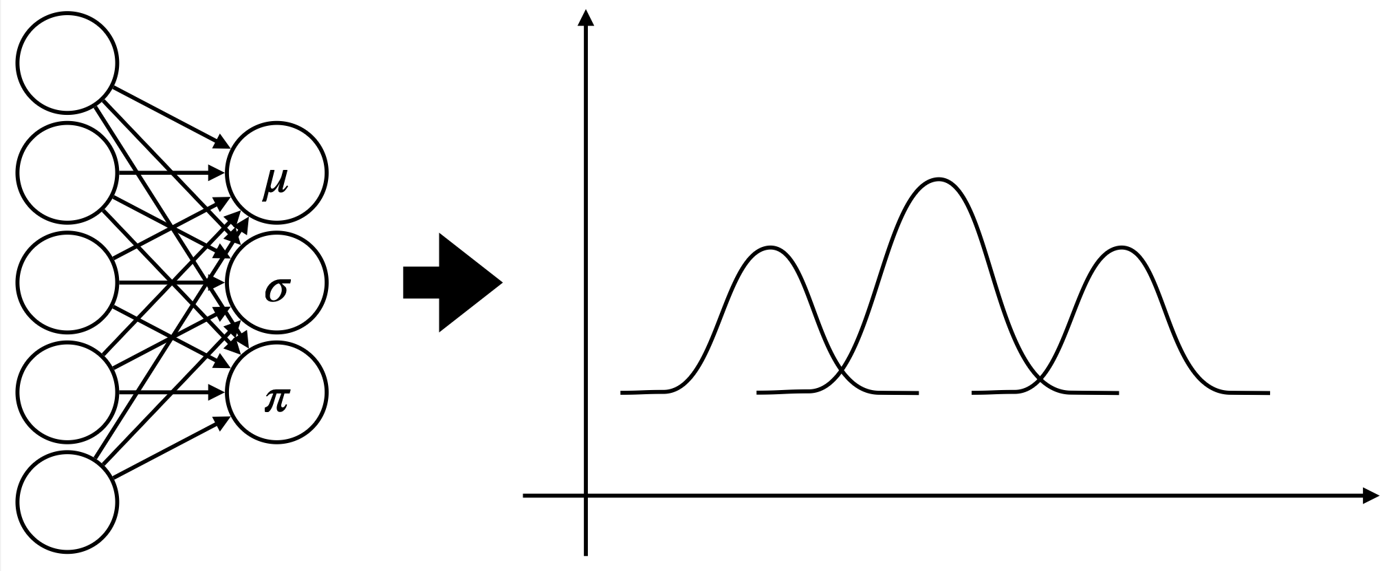
MDN: A Distribution-Predicting Neural Network

Mixture Density Networks address this by predicting not a single output, but a probability distribution over outputs.

Given input $\mathbf{x}$, an MDN predicts the parameters of a mixture of Gaussians:

$p(\mathbf{y} \mid \mathbf{x}) = \sum_k \pi_k(\mathbf{x}) · N(\mathbf{y} \mid \mu_k(\mathbf{x}), \sigma_k(\mathbf{x})^2)$

Where:

• $\pi_k(\mathbf{x})$: the mixing coefficients (probability of each mode)
• $\mu_k(\mathbf{x})$: the mean of each mode
• $\sigma_k(\mathbf{x})$: the standard deviation (uncertainty) of each mode

This formulation allows the model to learn multiple plausible outcomes and their associated likelihoods — crucial for stochastic systems.

---

Example: Modeling Physical Trajectories

Imagine modeling the next position of a bouncing ball given its current state. Depending on initial conditions and hidden factors (surface friction, elasticity, angle), the ball might:

• Bounce high,
• Skid and bounce low,
• Or roll without bouncing at all.

An MDN can represent these possibilities as distinct modes in its output distribution — each with its own probability and uncertainty — without collapsing them into an average that would be physically implausible.

---

Why MDNs Are Well-Suited for Natural Dynamics

MDNs shine in natural systems modeling for several reasons:

• Multi-modality: They can represent multiple likely outcomes from the same input.
• Uncertainty-aware: They learn both where the model is uncertain and how much.
• Smooth generalization: Because the mixture parameters are continuous, the model generalizes well to intermediate or novel states.
• Non-deterministic prediction: Ideal for simulation and planning where randomness is part of the process.

---

When Should You Use MDNs for Dynamics?

You should consider MDNs when:

• You expect multiple possible futures from a single state.
• You want to generate samples from learned dynamics (e.g. stochastic simulation).
• You’re modeling real-world systems where noise, randomness, or unobserved variables play a role.
• You need your model to output uncertainty-aware predictions, not just mean estimates.

---

Summary

Mixture Density Networks offer a principled way to model uncertain, multi-modal dynamics — a property that makes them particularly powerful for representing complex systems found in nature. When deterministic models fall short, MDNs can provide a richer, more realistic understanding of how the world behaves.

← To Profile